
Performance Measurement and Asset Management
The overall purpose of performance measurement is to help us select an investment and provide ongoing information about how our investment is doing so we can make good decisions about what to do next—both as an investor and as a money manager. In the course of everyday life, we often apply some kind of performance measurement and evaluation. When looking to a buy a car, for instance, it’s important to know how many miles per gallon it gets (or how far it can travel on a full charge), the length of the warranty, and what is actually covered under the warranty. To investigate all our options, the salesperson would probably share details about several models in the showroom. Plus, I would expect them to be knowledgeable about how that information compares with the competition at other dealerships.
It is no different when it comes to investing. That is, you can create and apply a basic framework for analyzing an investment that allows for informed decision-making.
A Note on Data Quality
Quality data inputs are critical to calculating accurate and reliable results. Data is typically gathered and stored on a daily basis and may include inputs from a trading, accounting, and performance measurement system. Some systems have all those components, while others comprise separate software packages that are integrated to create a whole.
The volume of data can be quite significant when you consider the number of portfolios, types of securities, different exchange rates, purchases and sales by the portfolio manager, contributions and withdrawals by clients, and the many types of transactions that get posted to each account.
The quality of the output is based on the quality of the inputs. As the saying goes, “If you put garbage in, you’ll get garbage out.”
Rate of Return Calculations
There are two acceptable ways to calculate a rate of return according to GIPS Standards (more on the standards later), depending on what we are trying to measure.
The first method is to calculate a time-weighted rate of return (TWRR), which ignores the impact of cash flows. This is ideal when we want to evaluate how a money manager is doing when they do not control the cash flows. There are approximation methods for the TWRR, but they can get distorted when there are large cash flows or when the returns are volatile.
We will look at an exact TWRR calculation that’s done on a daily basis and then geometrically linked for the entire period. The inputs we need are the beginning and ending value, the cash flows and how we want to weight them. The general formula is:

Let’s look at an example for a two-day period where we start with $100 and there are no cash flows. At the end of the first day, the account value is $105 or a return of 5.00%, and the second day value goes from $105 to $120 or a return of 14.29%. To get the return for both days, we geometrically link the individual days for a total return of 20.00%.

However, if we make a contribution of $3 on the second day, it is important for us to know how that cash flow should be weighted. Do those dollars get invested right away and participate in the market for the entire day (fully weighted) or do those dollars get invested at the very end of the day (zero weighted)?
A third option is to half-weight the cash flow if the timing of the investment varies. These settings can be made in a performance system and should be applied consistently. Here is a comparison of the three ways to apply the cash flow to the second day:
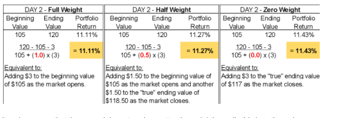
It makes sense that the second day return (no matter the weighting policy) is less than when there was no contribution, because the $3 increase to the portfolio was not due to the investment results of the money manager. The differences in returns in each of these cases reflects that the money manager was only responsible for the performance of the additional contribution from the time it was deemed to be participating in the market.
When a money manager does have control over the cash flows, it is important that we calculate a money-weighted rate of return (MWRR) to capture their impact. The general formula for the MWRR is shown below and solved by iteration:

Let’s assume we have $100,000 to invest and we invest our money with Carla, who manages a small-cap value strategy called Fund XYZ. We invest for two years; the return for year one is -90% and the return for year two is 50%.
If we use the TWRR, which neutralizes the impact of any cash flows, the result is -85%. However, if we gave Carla control over when to invest our money and she put $25,000 into the fund the first year and the remaining $75,000 into the fund at the beginning of the second year, we’d need to use the MWRR to measure Carla’s performance.
At the end of the first year, we would have lost -90% on $25,000, leaving us with $2,500. Carla then added $75,000, so the second year started with $77,500; after a return of 50%, we end up with $116,250. The result of the MWRR, which includes the impact of the cash flow, is 12.68%.
This is more intuitive, since we know the investment made money and Carla rightfully gets credit for the decision of when to deploy money into Fund XYZ.
Absolute, Benchmark, and Peer Comparisons
Once the returns are calculated, there are a few ways we can put them into context to help us make decisions about our investment. Let’s say we determine that $5,000,000 will allow us to retire comfortably and to achieve that goal, we invest with Carla in Fund XYZ. When we check our balance periodically and see that it’s on target, we’re probably happy that things are going in the right direction on an absolute basis. But we also want to know that we made a good decision by not passing up on better opportunities.
An investment generally has a stated benchmark, which is a reasonable starting point for a comparison if it meets certain criteria. To have any sort of meaning, the benchmark should be chosen ahead of time, be of a similar investment style, and also be applied consistently across periods. Provided this is the case, if we compare our returns to those of the benchmark and find we are ahead by some margin, then we typically feel better about the results.
We also want to examine the returns of investments that we do not own to see that we are not lagging on a relative basis. This can be accomplished by looking at our investment peers (other funds that have a similar strategy).
Companies like Morningstar and Thomson Reuters (Lipper) aggregate data from many different investment firms in order to create groupings of similar investment styles for comparison. Such companies publish information online and offer products with much more depth, including statistics, rankings, ratings and other tools to analyze individual investments and classes of investments. Comparing several metrics of an investment to its peers for various periods can be a very useful decision-making tool.
Risk and Risk-Adjusted Measures of Performance
It is very helpful to look at comparisons of investment returns, but that’s only half the story—the other half is the risk that was taken to achieve those returns. While there are many objective risk measures and statistics, the decision about how much risk is acceptable is very personal.
We may determine that an aggressive investment with a high degree of risk is suitable because we have a long time before we’ll need those funds. However, if we are going to get an ulcer from watching the ups and downs of the market, then perhaps a lower-risk investment would be more appropriate.
One way to measure the risk of an investment is to measure the variability of historical returns. A very common measure of stand-alone risk is an investment’s standard deviation. If two investments have the same return but one has a higher standard deviation, the preference would be for the one with the lower standard deviation, which indicates a manager is a more consistent performer.
Beta is another common statistic that measures an investment’s historical return relative to a benchmark. Figure 1 shows a scatter plot of investment returns versus benchmark returns over time. The slope of the best-fitting line using linear regression is the beta. When used to predict future returns, beta is essentially a multiple of how an investment’s return should move in relation to that of a benchmark. In this example, the beta of 1.1 means that on average, when the benchmark had a return of 1.00%, the investment had a return of 1.10%.

Figure 1
Measures like standard deviation and beta are used as a proxy for risk in calculating risk-adjusted measures of return. One of the most common measures is the Sharpe Ratio, which is a portfolio’s return in excess of the risk-free rate divided by the standard deviation of the portfolio. This measure tells us the ratio of reward per unit of risk: the higher the number the better.

Another risk-adjusted performance measure is the Information Ratio, which considers the “active return” to be the average difference between the investment return and the benchmark return. It is the variability (using the standard deviation) of the difference between the investment return and the benchmark return that is considered the “active risk.”

Equity Attribution
As the money manager of Fund XYZ, Carla is also interested in reviewing her performance because she knows that beating the benchmark and ranking well among her peers will help attract new clients.
One way to examine the portfolio is to look at the impact each investment’s contribution had on the total portfolio. This can be done with individual securities or groupings such as economic sectors, industries, or countries and shows how the fund did on an absolute basis.
The three tables that follow reflect a typical attribution report—they are identical except for the highlighted areas for discussion purposes. In Table 1, Fund XYZ and the benchmark are broken down into four industries with information for the fund presented first, then the benchmark, followed by attribution figures. Column C displays each group’s contribution to return. Specifically, the product of the weight and total return of Fund XYZ (columns A and B) will give us the contribution to return for each industry and the sum of those industries will equal the total return.
So what does this tell us about the fund? Looking at the contribution to return for the fund by itself, it is clear that investments in Food Wholesale and Food Retail made up the majority of the fund’s return, while the two other industries dragged down performance because 55% of the fund had a return between 1% and 3%.

The contribution to return for the benchmark can be analyzed in the same way, but it is generally included as a reference since the benchmark is directly part of the attribution analysis. The idea of an attribution model is that it should follow the investment decision making process, which includes deciding how much to allocate to each industry and then picking individual stocks within those industries.
One of the most common equity attribution models is the Brinson-Fachler model, which compares the fund to the benchmark in several ways to decompose the difference in total return. Column F in Table 2 is the allocation effect, which speaks to the impact of deciding to invest in a specific industry. If a particular industry outperformed within the benchmark (i.e., its return surpassed the benchmark’s overall return), then what was the impact of the money manager’s industry allocation decision to over- or underweight versus the benchmark?
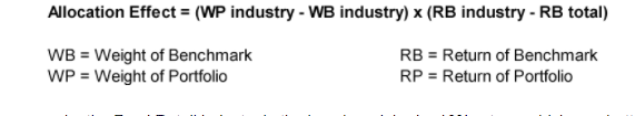
For example, the Food Retail industry in the benchmark had a 10% return, which was better than the total benchmark’s return of 9.35%, and the fund was overweight this industry versus the benchmark. The positive allocation effect of 0.03% indicates this was a good investment decision.
A positive allocation effect can also be achieved by underweighting an industry whose benchmark return was lower than the benchmark’s total return, such as in Electronics. The positive allocation of 0.07% indicates it was a good decision to underweight an underperforming industry.

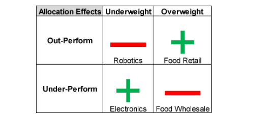
The other two possibilities of overweighting an underperforming industry and underweighting an outperforming industry are reflected in Food Wholesale and Robotics, respectively. The four possibilities for the allocation effect are shown in the table below:
The allocation effect addresses the group-level investment decision of which industries to invest in, but the selection effect tells us how the manager did at picking individual stocks within those groups. Column G in Table 3 is the selection effect and answers the following question: If Fund XYZ had the same industry weight as the benchmark, which return was better?
The Fund’s 12% return in Food Retail is better than the benchmark’s 10% return and the positive selection effect of 0.20% indicates good stock-picking decisions. On the other hand, Fund XYZ’s return of 3% in Robotics compared to the benchmark’s 11% is reflected in the large negative selection effect of -3.60%.

Column H is the interaction effect; it’s often debated what this represents, since it does not isolate the impact of the weights or returns in the formula and is not directly mapped to the investment decision making process. It is calculated as the difference in weights between the fund and the benchmark multiplied by the difference in returns between the fund and the benchmark. It is necessary to obtain the total effect, but it’s most often combined with either the allocation effect (for managers with a top-down, macro approach) or the selection effect (for managers with a bottom-up, stock-picking approach).
In combination, understanding the allocation, selection, and interaction effects can provide deeper insight into the factors driving the performance of a portfolio of investments versus its benchmark. This type of attribution analysis has been increasingly used by sophisticated investors (i.e., endowments, pension funds) to evaluate and monitor the money managers they hire on behalf of their respective beneficiaries.
GIPS Standards
A general discussion of performance measurement would not be complete without mentioning the Global Investment Performance Standards (GIPS) created by the CFA Institute. These are a set of voluntary standards based on the idea that performance results should be presented fairly and with full transparency in order to promote comparability.
These standards provide clarity on what is required to comply with the standards, as well as recommendations for best practices. In addition to explaining the various provisions of GIPS (such as calculation methodology, composite construction, presentation and reporting, disclosures, etc.), the standards also include detailed guidance statements to assist in their interpretation and application.
This level of standardization promotes integrity and enables investors to do an apples-to-apples comparison of performance results in order to make more informed investment decisions. The GIPS standards have evolved over the years and continue to do so in tandem with industry changes.
About the Author

Philip Delin joined International Value Advisers, LLC (IVA) in June 2013 as an investment performance analyst. He is responsible for performance measurement reporting, risk analytics, and maintaining GIPS compliance. Prior to joining IVA, Philip worked as a senior analyst in the financial planning group at Bank Leumi. Before joining Leumi in 2010, Philip was head of the performance analytics group at Columbia Management.
Philip earned a B.S. in business from SUNY Buffalo and an MBA from Pace University. He holds the Chartered Financial Analyst (CFA) and Certificate in Investment Performance Measurement (CIPM) designations.